


Overall Robot
Here, a thorough explanation of every element of their Simscape model, the technical drawing of the robot and the exploded view of the wheel-legged biped robot is given. They offered a thorough explanation of the responsibilities and purposes of each component in the model, going over each one step by step.
Technical Drawing
The technical drawing of a Solidworks model of a wheel-legged biped robot provides detailed information about the size, shape, and geometric characteristics of the robot's components. In the case of a wheel-legged biped robot, technical drawings would be used to communicate the design and dimensions of the robot's components to manufacturers or other stakeholders. This drawing is created by selecting appropriate views of the robot, adding dimensions and annotations to indicate the size and location of the components, and specifying tolerances to ensure accurate and consistent manufacturing. Additionally, a bill of materials is included to list all the components and their respective part numbers, quantities, and descriptions. The technical drawing plays a crucial role in communicating the design and dimensions of the robot to manufacturers or other stakeholders, ensuring that it can be manufactured accurately and assembled correctly. The technical drawing of the Solidworks model of a wheel-legged biped robot is an essential tool for optimizing the manufacturing process and ensuring the quality and functionality of the final product. This plays an important role in ensuring that the robot can be manufactured accurately and assembled correctly. By providing detailed information about the design and dimensions of the robot's components, these drawings help to minimize errors and improve the efficiency of the manufacturing process.

Exploded View
An exploded view of a SolidWorks model of a wheel-legged biped robot shows how the components of the robot fit together and interact with one another. It is created by separating the individual components of the robot and positioning them in their relative positions to show how they fit together. This view is typically used in assembly instructions to help technicians and manufacturers to understand how to assemble the robot correctly. In an exploded view of a wheel-legged biped robot, each component is shown with its own set of dimensions and annotations, allowing for easy identification and assembly. Additionally, each component is labelled with a part number, enabling easy referencing in the assembly instructions.
By visualizing the individual components of the robot in an exploded view, technicians and manufacturers can better understand how each part interacts with the others, and ensure that they are assembled in the correct order and orientation. This view is also useful for identifying potential problems or issues in the design, allowing for adjustments to be made before the manufacturing process begins. The exploded view of a Solidworks model of a wheel-legged biped robot provides a clear and detailed visual representation of the robot's components, facilitating efficient and accurate assembly and ensuring the quality and functionality of the final product.
-
Torque
In Simulink and Simscape, torque is a physical quantity that represents the rotational force applied to an object, in this case, the wheel-legged biped robot. Torque is essential to modelling the dynamics of the robot's motion, especially for simulating the effects of gravity, friction, and other external forces on the robot's movement.
For the wheel-legged biped robot, torque is used to control the robot's joint motors, which in turn control the motion of the robot's limbs. The torque produced by the motors is proportional to the current applied to them, and the direction of the torque determines the direction of the joint movement. In Simulink and Simscape, the torque required to move a joint can be calculated based on the mass, acceleration, and other physical properties of the robot, as well as the external forces acting on it. The control system of the robot can then use this information to determine the appropriate amount of torque to apply to each joint, in order to achieve the desired motion. Torque plays a crucial role in the simulation of the wheel-legged biped robot's motion in Simulink and Simscape, as it allows for accurate modelling of the robot's dynamics and control of its movement.
-
Position
In Simulink/Simscape, position refers to the location of a physical component in space, relative to a reference frame. In the case of a wheel-legged biped robot, the position can be described using three coordinates that represent the location of the robot's centre of mass in the x, y, and z directions.
These positions can be measured using sensors or estimated using mathematical models. In Simulink/Simscape, the position of a component can be specified using the appropriate blocks such as the Joint blocks or the Transform block.
For example, in a wheel-legged biped robot, the position of the knee joint can be specified using the Revolute Joint block or the Prismatic Joint block. The position of the robot's centre of mass can be estimated using the Rigid Transform block to combine the positions of the individual components.
The position of the robot can also be controlled using actuators such as motors or hydraulic systems. The desired position can be specified using input signals to the appropriate blocks, such as the Actuator blocks. Accurate position control is important for the proper functioning of a wheel-legged biped robot, as it determines the robot's movement and stability.
-
Friction
The frictional force between the wheels of your robot and the ground will depend on several factors, including the surface material, the weight of the robot, and the design of the wheels. Here are some general guidelines and values for frictional force that you can use as a starting point:
Static friction: The maximum amount of static friction is equal to the normal force times the coefficient of static friction, μ_s. The coefficient of static friction will depend on the materials in contact. For example, the coefficient of static friction between rubber and concrete is typically around 0.7.
Dynamic friction: The force of dynamic friction is typically lower than the maximum static friction and is proportional to the normal force times the coefficient of dynamic friction, μ_d. The coefficient of dynamic friction is typically lower than the coefficient of static friction and will depend on the specific materials in contact. For example, the coefficient of dynamic friction between rubber and concrete is typically around 0.4.
It is important to note that these values are general guidelines, and the specific values for your robot may be different. You will need to experiment with different values to find the optimal frictional force for your robot.
-
Angles
In Simulink, the angles of the robot for a wheel-legged biped can be modeled using the Joint blocks, such as the Revolute Joint, Planar Joint, and 6-DOF Joint blocks. These blocks provide the rotational degrees of freedom needed to define the angles of the robot's joints.
For example, the Revolute Joint block models a joint that has one rotational degree of freedom. It defines the angle of rotation between the base and follower frames. Similarly, the Planar Joint block provides one rotational and two translational degrees of freedom between two frames. It can be used to model joints that move in a plane, such as the hip and shoulder joints of the robot.
The 6-DOF Joint block provides three translational and three rotational degrees of freedom, and can be used to model complex joints, such as the ankle joint of the robot, which has both rotational and translational degrees of freedom.
In general, the angles of the robot's joints can be defined as input signals to the Joint blocks, and the outputs of these blocks can be used as inputs to other blocks in the Simulink model, such as the Motor blocks, to generate torques that drive the motion of the robot.
The description of every element in their Simscape model of a biped robot with wheels. Each element is thoroughly broken down in the post, with an explanation of its purpose and place in the model. The article gives a thorough rundown of all the significant Simscape model elements for the biped robot with wheels. Each component is thoroughly explained in the section above, emphasising its significance and role in the overall design.
Simscape Model
The entire concept of each component of the wheel-legged biped robot in the Simscape model has been thoroughly described and elaborated on.
-
Mechanical configuration
The Mechanism Configuration block is a key component in Simscape Multibody that specifies the gravity and simulation parameters of the mechanism. This block is used to set the physical properties of the mechanism, such as the strength and direction of the gravitational field, as well as the simulation parameters that affect how the mechanism behaves.
The gravitational field is an important physical property of the mechanism that affects its motion and behavior. The Mechanism Configuration block allows you to specify the strength and direction of the gravitational field by setting the Uniform Gravity parameter. This parameter specifies the magnitude of the gravitational acceleration, in meters per second squared, acting on all components in the mechanism.
In addition to setting the physical properties of the mechanism, the Mechanism Configuration block also allows you to specify simulation parameters that affect how the mechanism is simulated. One of the most important simulation parameters is the perturbation value, which is used to compute numerical partial derivatives during linearization. This value affects the accuracy of the simulation, and must be set carefully to ensure accurate results. Another important simulation parameter is the iteration number for the joint mode transition. This parameter determines how many iterations are performed during the transition between different joint modes, which can affect the stability and accuracy of the simulation.
It is worth noting that a Simscape Multibody network can have at most one instance of the Mechanism Configuration block. If a model does not have the Mechanism Configuration block, the uniform gravity applied to the mechanism is zero. If a network contains a Gravitational Field block, the Uniform Gravity parameter of the block should be set to None, to avoid double-counting the gravitational field. The block is a crucial component in Simscape Multibody that allows you to specify the physical properties and simulation parameters of the mechanism. By setting these parameters carefully, you can ensure that your simulation accurately models the behavior of your mechanism, and can analyze its motion and behavior under a wide range of conditions.

-
Solver configuration
-
The Solver Configuration block is an essential component of Simscape that specifies the solver parameters needed for simulation of a physical network represented by a connected Simscape block diagram. This block contains settings that determine the behaviour and accuracy of the simulation. In Simscape, a physical network is represented by a connected block diagram, which includes different components such as sources, sensors, actuators, and physical systems. To simulate the behaviour of such a network, it is necessary to specify solver settings, which are used to determine the step size, tolerance levels, and other parameters of the simulation.
-
The Solver Configuration block is used to specify these solver settings for the physical network. This block contains a number of parameters that can be set to control the behaviour of the simulation, including the solver type, the solver algorithm, and the step size. The solver type specifies the type of solver that is used for the simulation. Simscape supports several different solver types, including fixed-step and variable-step solvers. Fixed-step solvers use a fixed step size for each simulation time step, while variable-step solvers adjust the step size dynamically to maintain a specified level of accuracy. The solver algorithm determines how the solver performs the simulation. There are different algorithms available in Simscape, such as explicit and implicit solvers. The choice of algorithm depends on the nature of the physical system being simulated and the accuracy requirements of the simulation.
-
The step size parameter determines the size of the time step used by the solver during the simulation. This value can be set to a fixed value for fixed-step solvers, or can be automatically adjusted for variable-step solvers. It is important to note that each topologically distinct Simscape block diagram requires exactly one Solver Configuration block to be connected to it. This block is necessary to specify the solver settings for the simulation, and is required for the simulation to run correctly.

-
World
-
The World Frame block in Simscape Multibody provides access to the global reference frame or ground frame in a mechanical model. This frame is inertial and at absolute rest, with orthogonal and right-handed coordinate axes arranged according to the right-hand rule. It is the ultimate reference frame in a frame network, with all other frames defined directly or indirectly with respect to it. All frame ports connected to the World Frame block or indirectly connected through other frame ports identified with the World frame are also identified with the World frame. In a frame network, the World frame is the ultimate reference frame. Directly or indirectly, all other frames are defined with respect to the World frame. If multiple World Frame blocks connect to the same frame network, those blocks identify the same frame. If no World Frame block connects to a frame network, a copy of an existing frame, frozen in its initial position and orientation, serves as the World frame.
-
A model can have multiple World Frame blocks, but they all represent the same frame. If no World Frame block connects to a frame network, a copy of an existing frame, frozen in its initial position and orientation, serves as the World frame.

-
PID Controller
The PID Tuner is a tool in Simulink that provides a fast and widely applicable single-loop PID tuning method for the PID Controller blocks. This tool allows users to tune PID controller parameters to achieve a robust design with the desired response time. The typical design workflow with the PID Tuner involves the following tasks:
-
Launching the PID Tuner: When launching the PID Tuner, the software automatically computes a linear plant model from the Simulink model and designs an initial controller. The computed plant model represents the linearized version of the Simulink model, which is used by the PID Tuner to design the controller.
-
Tuning the controller: The user can tune the controller in the PID Tuner by manually adjusting design criteria in two design modes, namely the time-domain and frequency-domain modes. The tuner computes PID parameters that robustly stabilize the system by meeting the design criteria set by the user. The user can also validate the controller design by simulating the closed-loop system and observing its behaviour.
-
-
Exporting the controller parameters: Once the user is satisfied with the controller design, they can export the parameters of the designed controller back to the PID Controller block in the Simulink model. The exported parameters will replace the initial controller design computed by the PID Tuner. The user can then verify the controller performance in Simulink by simulating the closed-loop system and observing its behaviour.
The PID Tuner is a powerful tool that allows users to tune PID controller parameters quickly and efficiently by providing an easy-to-use interface for designing and validating controllers. It is widely used in industries and academia to achieve robust and stable control of various dynamic systems.
Proportional Gain, Integral Gain, and Derivative Gain are the three main parameters used in a Proportional-Integral-Derivative (PID) controller, which is a common type of feedback control used in various engineering applications. The PID controller aims to achieve a desired output by continuously adjusting a control signal based on the error between the desired output and the actual output.
-
Proportional Gain (Kp): This is the primary gain parameter in the PID controller, and it is proportional to the error signal. Increasing the proportional gain results in a faster response to changes in the error signal. However, if the gain is too high, the system may become unstable and oscillate around the desired setpoint. On the other hand, if the gain is too low, the system may not respond fast enough to changes in the error signal, resulting in a sluggish response.
-
Integral Gain (Ki): This gain parameter considers the accumulated error over time and is proportional to the integral of the error signal. The integral gain helps to reduce steady-state errors in the system. It also helps to eliminate the effects of external disturbances that may affect the system's performance. However, if the integral gain is too high, it can cause the system to become unstable and oscillate around the setpoint.
-
Derivative Gain (Kd): This gain parameter is proportional to the derivative of the error signal and helps to reduce overshoot and dampen oscillations. The derivative gain is used to anticipate future trends in the error signal and to prevent overshoot or undershoot. However, if the derivative gain is too high, it can amplify high-frequency noise in the system and cause instability.
The proportional gain adjusts the controller's response to the current error signal, the integral gain adjusts the controller's response to the accumulated error over time, and the derivative gain adjusts the controller's response to the rate of change of the error signal. The optimal values for these gains depend on the system's characteristics and the desired performance. The PID Tuner tool in Matlab and Simulink can be used to find the optimal values for these gains for a given system.
-
Add, subtract, sum of elements, sum
The Sum block in Simulink performs mathematical addition or subtraction operations on its input signals. The block can handle scalar, vector, or matrix inputs and can also perform a summation of signal elements. The Sum block is also known as the Add, Subtract, Sum of Elements, or simply the Sum block.
The Sum block has a single output port and multiple input ports. Each input port is identified with a plus (+) or minus (-) sign, which specifies whether the input is to be added or subtracted from the total. You can use the List of signs parameter to specify the operation for each input port, and you can use the Spacer (|) sign to create a blank space in the list of signs. The Sum block can perform different types of mathematical operations depending on the input signals. For scalar inputs, the block performs basic arithmetic addition or subtraction. For vector or matrix inputs, the block performs element-wise addition or subtraction of corresponding elements. If the input signals have different dimensions, the block automatically pads the smaller signals with zeros to match the larger signal.
The Sum block can also perform a summation operation on the elements of a signal. To do this, you need to select the Sum of Elements option in the block parameters. The block then adds all the elements of the input signal along the specified dimension, which can be either the row or column dimension.

-
Gain
-
The Gain block in Simulink is used to multiply the input signal by a constant value, which is referred to as the gain. The input and gain values can be scalar, vector, or matrix. The block has a single input port and a single output port. The input signal is multiplied by the gain value, and the resulting product is sent to the output port of the block.
-
The Gain block's gain value is set in the Gain parameter. You can specify the value directly or use a signal to set the gain value dynamically during the simulation. The Multiplication parameter of the Gain block lets you specify whether to perform element-wise multiplication or matrix multiplication. For matrix multiplication, this parameter also lets you indicate the order of the multiplicands. When the simulation runs, the gain value is first converted from double to the data type specified in the block mask. The input signal is then multiplied by the gain value, and the resulting product is converted to the output data type using the specified rounding and overflow modes.
-
The Gain block is used in various control systems applications to amplify or attenuate signals before feeding them into a controller. For example, in a PID (Proportional-Integral-Derivative) controller, the proportional gain is set using the Gain block to adjust the strength of the feedback control signal. By varying the gain value, the controller's response to the error signal can be adjusted to achieve the desired system response.

-
Goto tag
The Goto block and its corresponding From block are used in Simulink to pass signals between blocks without physically connecting them. The Goto block receives an input signal from another block in the model, which it then sends to any corresponding From blocks. The Goto block can pass its input signal to multiple From blocks, but each From block can only receive signals from one Goto block. The Goto block and its corresponding From block must have the same tag name, which is used to identify the connection between them.
To specify the tag name for the Goto and From blocks, you can double-click on the block and enter the tag name in the Tag field. If the tag visibility is set to "scoped", then you also need to use a Goto Tag Visibility block to define the visibility of the tag.
The Goto block can receive input signals of any data type, including real- or complex-valued signals or vectors. The input signal is multiplied by a gain value of 1 by default, but the gain can be adjusted by changing the Gain parameter in the block's dialog box. The Goto block provides a convenient way to pass signals between blocks in a Simulink model without having to physically connect them, which can make the model easier to read and understand.

-
From tag
The From block is a Simulink block used in Simscape networks to extract a physical signal from a network and make it available as a Simulink signal for further processing. When you place a From block in a Simscape diagram, it creates an output port that corresponds to the physical signal being extracted. You can then connect this output port to other Simulink blocks to further process the extracted signal. The From block also has a dialog box where you can set the block's label and other properties.
The From block is usually used in conjunction with the Goto block. The Goto block sends a signal to the corresponding From block, allowing you to pass a signal from one Simscape block to another without directly connecting them. The From block receives the signal sent by the Goto block and makes it available as a Simulink signal.
In addition to its basic functionality of extracting a physical signal, the From block can also perform several other operations on the signal. For example, you can use the From block to display a signal's minimum or maximum value, or to display a signal as a bar graph or XY plot. The block can also perform mathematical operations such as adding, subtracting, or multiplying signals. The From block is a fundamental Simscape block used to extract a physical signal from a network and make it available as a Simulink signal for further processing. It is often used in conjunction with the Goto block to pass signals between Simscape blocks.

-
Simulink-PS Convertor
The Simulink-PS Converter block is a Simscape block that allows the conversion of a Simulink signal into a physical signal that can be used as an input to a Simscape physical network. This block acts as an interface between the Simulink environment and the Simscape environment.
This block has a single input port that accepts a Simulink signal, and a single output port that provides a physical signal that can be connected to other Simscape blocks. The input signal can be of any Simulink data type, such as scalar, vector, or matrix. The Simulink-PS Converter block automatically converts the Simulink signal into a physical signal that has the appropriate units for the corresponding Simscape domain. For example, if the physical system is modelled in the mechanical domain, the input signal units should be in newton-meters (Nm) for torques and in meters (m) for distances.
Once the Simulink signal is converted into a physical signal, it can be connected to other Simscape blocks to form a physical network. The physical network can then be simulated using the Simscape solver to obtain the system's behaviour over time.

-
PS-Simulink Convertor
Photo
The opposite of the Simulink-PS Converter block is the PS-Simulink Converter block. It transforms a SimscapeTM physical network's physical signal into a Simulink signal. You can use this block to link Simulink scopes, displays, and other Simulink blocks to Simscape models.
When you want to track the simulation outcomes of a Simscape model in a Simulink display block, the PS-Simulink Converter block is helpful. It enables you to view and examine the simulation output of the Simscape-modeled physical system. One physical signal input port on the PS-Simulink Converter block accepts physical signals from the Simscape physical network. A Simulink signal is created from the physical signal by the block and is then made available at the output port. The output signal can be used as an input to any Simulink block or scope.
When you connect the PS-Simulink Converter block to a physical network, you can specify the units of the physical signal using the Units parameter. The Units parameter ensures that the units of the physical signal match the units expected by the Simulink block to which the PS-Simulink Converter block is connected.
-
Step
The Step block in Simulink is a type of signal generator block that provides a step between two definable levels at a specified time. The block has two input parameters: the Step time and the Final value. If the simulation time is less than the Step time parameter value, the block's output is the Initial value parameter value (default is zero). For simulation time greater than or equal to the Step time, the output is the Final value parameter value.
The Step block can be used to simulate the behaviour of a system that experiences a sudden change in input, for example, a switch turning on or off, or a valve opening or closing. The block can be used to generate a step input signal of specified amplitude and duration.
The numeric block parameters must be of the same dimensions after scalar expansion. The user can specify the interpretation of vector parameters by turning on or off the Interpret vector parameters as 1-D option. If the Interpret vector parameters as 1-D option is off, the block outputs a signal of the same dimensions and dimensionality as the parameters. If the Interpret vector parameters as 1-D option is on and the numeric parameters are row or column vectors (that is, single-row or column 2-D arrays), the block outputs a vector (1-D array) signal. Otherwise, the block outputs a signal of the same dimensionality and dimensions as the parameters.

-
Scope
The Time Scope is a tool used in Simulink to display signals generated during simulation in a graphical format. The tool allows you to visualize signal waveforms, making it easier to monitor system behaviour and diagnose problems.
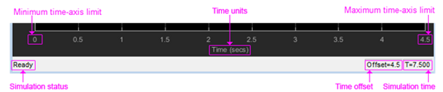
The Time Scope has two important parameters, the Time span and Time display offset, which determine the time range of the signals displayed on the scope window. The Time span parameter specifies how much simulation time to display at a time, while the Time display offset parameter determines the start time of the displayed signals. For example, if the Time span is set to 25 seconds and the Time display offset is set to 5 seconds, the scope will display 25 seconds' worth of simulation data from 5 to 30 seconds on the time axis. To change the display settings of the signals on the Time Scope, you can access the Configuration Properties dialog box by selecting View > Configuration Properties. In this dialog box, you can modify the Time span and Time display offset parameters, as well as other display settings such as the plot colours and grid style.
The Time Scope also includes indicators that communicate information about the simulation time and the displayed signals. The Time units indicator displays the units of the time axis, which can be set to seconds, milliseconds, or microseconds. The Time offset indicator displays the start time of the displayed signals, and the Simulation time indicator displays the current simulation time.
-
Revolute joint
The Revolute Joint block in Simulink and Simscape is used to model a joint that has one rotational degree of freedom. It is a fundamental building block for modelling mechanical systems that involve rotational motion.
The Revolute Joint block has two physical connection ports labelled A and B, which are used to connect other physical elements in a Simscape model. The rotational degree of freedom is modelled as the rotation of a shaft that is connected between the two ports. The shaft can rotate about its axis, and the rotation is measured in radians.
The block has several parameters that can be used to customize its behavior. These include:
-
Initial position: specifies the initial angle of the joint when the simulation starts
-
Initial velocity: specifies the initial angular velocity of the joint when the simulation starts
-
Upper limit: specifies the maximum allowable angle of rotation for the joint
-
Lower limit: specifies the minimum allowable angle of rotation for the joint
-
Stiffness: specifies the rotational stiffness of the joint
-
Damping: specifies the rotational damping of the joint
The Revolute Joint block can be used in a wide range of mechanical systems, including robotic arms, vehicle suspensions, and machinery with rotating components. Its simple design and customizable parameters make it a powerful tool for modelling complex mechanical systems in Simulink and Simscape.

-
Cylindrical joint
The cylindrical Joint block in Simscape Multibody allows you to model a joint with one translational and one rotational degree of freedom. This block combines two primitive joints, a prismatic joint and a revolute joint, which are connected such that their translation and rotation axes remain aligned during simulation.
The joint provides the translational degree of freedom, which allows motion along a single axis, while the revolute joint provides the rotational degree of freedom, which allows rotation around an axis. The combination of these two joints provides a joint that has one translational and one rotational degree of freedom. You can specify the joint properties, such as joint limits and damping, through the block parameters. Additionally, you can connect the joint to other bodies in your model by specifying their frames of reference.
The cylindrical Joint block is commonly used to model joints in mechanical systems, such as robot arms or vehicle suspensions, that require both translational and rotational motion.
-
Reference frame
In a multi-body dynamics simulation, reference frames are used to define the position and orientation of bodies in the simulation. The Reference Frame block in Simulink/Simscape allows you to define a reference frame with respect to which you can define other frames. This reference frame is generally non-inertial and can accelerate with respect to the World frame.
The Reference Frame block is optional in a model, and if it is not present, the World frame is used as the reference frame. The block allows you to specify the initial position and orientation of the reference frame and also provides an interface for specifying the angular and linear velocities of the frame.
In a Simulink/Simscape model, the Reference Frame block is often used in conjunction with other blocks such as the Rigid Transform block or the Joint block to define the kinematics and dynamics of the system. By defining the position and orientation of frames with respect to the reference frame, you can define the position and orientation of bodies in the simulation.

-
Rigid transform
The Rigid Transform block is used to apply a fixed transformation between two frames in a Simscape Multibody system. The block has two input ports, a base port and a follower port, each representing a frame. The base port frame is the reference frame, and the follower port frame is the frame that is transformed with respect to the base frame.
The transformation between the base and follower frames is specified using rotation and translation parameters. The rotation can be specified as either Euler angles or a rotation matrix, and the translation can be specified as a vector. The block applies the transformation in a time-invariant manner, meaning that the transformation does not change over time during simulation.
It is important to note that the frames remain fixed with respect to each other during simulation and move only as a single unit. If you need to model a system with multiple rigid bodies, you can combine the Rigid Transform block with Solid blocks to create compound rigid bodies.

-
Planer joint
The Planar Joint block is a Simscape Multibody block that provides a connection between two frames, allowing for one rotational and two translational degrees of freedom between them. The two frames are called the Base Frame and Follower Frame, respectively.
The rotational degree of freedom is provided by a revolute joint between the frames. This joint allows the follower frame to rotate about the common axis of the joint with respect to the base frame. The translational degrees of freedom are provided by prismatic joints perpendicular to the common axis of the revolute joint. These joints allow the follower frame to translate along two orthogonal directions in the plane perpendicular to the common axis.
The Planar Joint block is commonly used to model systems with two-dimensional motion, such as robots that move in a plane or vehicles that move along a flat surface. To use the Planar Joint block, you must connect its Base Frame and Follower Frame ports to other frames in your model. You can then set the initial position and orientation of the follower frame with respect to the base frame, as well as the limits and damping for each degree of freedom. The block also provides options for modelling joint backlash and stiction, which can affect the dynamics of your system.

-
6-DOF Joint
The 6-DOF Joint block is a Simscape Multibody block that provides three translational and three rotational degrees of freedom between two frames. The follower frame can have a 3-D transformation with respect to the base frame. The transformation contains three sequential translations and a 3-D rotation encoded as a quaternion. Quaternions do not have a kinematic singularity, which makes them a popular choice for modelling 3-D rotations.
The block has two input ports and two output ports. The input ports are labelled "F" and "B", which correspond to the follower and base frames, respectively. The output ports are labelled "Fp" and "Bp", which correspond to the follower and base frame positions and orientations.
The block uses a 3-D transformation matrix to specify the position and orientation of the follower frame with respect to the base frame. The transformation matrix contains three sequential translations and a 3-D rotation encoded as a quaternion. The rotation part of the transformation is encoded as a quaternion because quaternions do not have a kinematic singularity.
The block parameters allow you to specify the initial position and orientation of the follower frame with respect to the base frame. You can also specify the range of motion for each degree of freedom and the limits on the forces and torques that can be applied to the joint. The 6-DOF Joint block is commonly used in Simscape Multibody models to connect rigid bodies with six degrees of freedom. For example, the block can be used to model the joints in a robotic arm or the suspension system in a vehicle.

-
Transform sensor
The Transform Sensor block in Simulink is used to measure the relative spatial relationship between two frames connected to its F and B ports. The block provides three output signals - Relative Pose, Relative Velocity, and Relative Acceleration - which are used to measure the relative position, velocity, and acceleration between the two frames.
To use the Transform Sensor block, the user must first define the frames that are to be connected to its F and B ports. The F port represents the follower frame, while the B port represents the base frame. Once the frames have been defined and connected to the respective ports, the block measures the relative spatial relationship between them.
The Relative Pose output signal provides the orientation and position of the follower frame with respect to the base frame. This signal is represented as a 4x4 homogeneous transformation matrix, which includes the orientation and position of the follower frame relative to the base frame. The Relative Velocity output signal provides the linear and angular velocities of the follower frame relative to the base frame. This signal is represented as a 6x1 vector, which includes the linear velocity and angular velocity components along the x, y, and z axes.
The Relative Acceleration output signal provides the linear and angular accelerations of the follower frame relative to the base frame. This signal is represented as a 6x1 vector, which includes the linear acceleration and angular acceleration components along the x, y, and z axes. It should be noted that the Transform Sensor block measures only the relative spatial relationship between the two frames. To measure the absolute translational or rotational quantities of a frame, the user must connect the frame to both the F and B ports of the block, where the B port is connected to the world frame of the model.

-
Integrator
In Simulink/Simscape, the Integrator block is used to perform integration of an input signal with respect to time. The output of the Integrator block is the integral of the input signal. Mathematically, the block computes the area under the curve of the input signal.
The Integrator block has one input port and one output port. The input port accepts the signal to be integrated. The output port provides the integrated result. The Integrator block can be used for both scalar and vector signals. The Integrator block has several parameters that can be used to configure its behaviour, including:
-
Initial condition: This parameter specifies the initial value of the integrated signal. By default, the initial condition is set to zero.
-
Integration method: This parameter determines the integration method used by the block. The default method is the "ode4 (Runge-Kutta)" method, which is a fourth-order Runge-Kutta method.
-
Maximum step size: This parameter sets the maximum step size used by the integrator. The default value is Inf, which means that there is no maximum step size.
It is important to note that the Integrator block can produce numerical errors, particularly when the input signal has sharp changes or when the integration time step is too large. To avoid these errors, it is recommended to use a fixed-step solver, such as the ode1 (Euler) solver, and to choose an appropriate time step size. Additionally, the use of a State-Space block, which can be more stable than the Integrator block, may be preferable in some cases.

-
Prismatic joint
In Simulink, the Prismatic Joint block models a connection that restricts the relative motion between two frames to one translational degree of freedom. This type of motion is common in hydraulic or pneumatic cylinders, which involve linear motion.
The Prismatic Joint block has only one prismatic primitive, which is along the z-axis of the base frame. During simulation, the z-axes of the base and follower frames align, and the follower frame moves with respect to the base frame along the z-axis. The block has two frame ports: the base port and the follower port. The base port is the reference frame, and the follower port moves relative to the base port. The Prismatic Joint block has two physical conserving ports: the translational port and the axial port. The translational port is the physical signal output port for the translational motion. It outputs the distance travelled by the follower frame along the z-axis with respect to the base frame. The axial port is the physical signal input port for the force that causes the translational motion. It is used to model the actuation mechanism for the joint, such as a hydraulic or pneumatic actuator.
The block parameters include initial position and velocity, lower and upper limits for the translational motion, and damping and stiction coefficients. The initial position and velocity parameters specify the starting position and velocity of the follower frame relative to the base frame. The limits parameters constrain the motion of the follower frame to lie within a specified range along the z-axis. The damping and stiction parameters model the resistance to motion of the joint due to friction.

-
Spatial Contact force
The Spatial Contact Force block in Simscape allows you to model the interaction between two solid objects in contact. This block can be used to simulate scenarios where two objects come into contact with each other, such as a ball bouncing off a surface or two objects colliding with each other. To use this block, you first need to specify the two solids that are in contact by connecting them to the corresponding Solid blocks. You can then choose between using the built-in penalty method or creating a custom contact force law to model the contact between the two solids.
The built-in penalty method assumes that the contact between the solids is smooth and continuous, and calculates the contact force using a penalty function that generates a force proportional to the depth of penetration between the two solids. The penalty function uses a spring-like behaviour to push the solids apart, ensuring that they remain in contact but do not interpenetrate. You can adjust the strength of the penalty force by modifying the block's parameters. Alternatively, you can create a custom contact force law that defines the relationship between the contact force and the depth of penetration. This can be useful when modelling contacts that do not follow the smooth, continuous assumptions of the penalty method, such as contacts that involve impact or sliding.
The Spatial Contact Force block also allows you to specify friction coefficients for the contact, which can affect the behaviour of the solids as they come into contact and slide against each other. These coefficients can be set to specific values, or you can choose to use default values that are calculated based on the materials of the solids.

-
Slider Gain
In Matlab Simulink, the slider gain block is a commonly used block that is used to change the gain of a signal dynamically during simulation. The slider gain block allows the user to define a gain value using a slider that can be adjusted during simulation, which is particularly useful for tuning control systems.
The slider gain block has a single input port and a single output port. The input signal is multiplied by the gain value, which can be adjusted using the slider. The output signal is the result of this multiplication. To use the slider gain block, the user needs to specify the minimum and maximum gain values, as well as the initial gain value. The user can also specify the step size of the slider, which determines the amount by which the gain changes when the slider is moved.
During simulation, the user can adjust the slider to change the gain value in real-time. This allows the user to quickly tune the gain of a control system and observe the effects of the changes on the system's behaviour. The slider gain block is a powerful tool for adjusting gain values during simulation and tuning control systems.

-
Spatial Contact force
The Spatial Contact Force block in Simscape allows you to model the interaction between two solid objects in contact. This block can be used to simulate scenarios where two objects come into contact with each other, such as a ball bouncing off a surface or two objects colliding with each other. To use this block, you first need to specify the two solids that are in contact by connecting them to the corresponding Solid blocks. You can then choose between using the built-in penalty method or creating a custom contact force law to model the contact between the two solids.
The built-in penalty method assumes that the contact between the solids is smooth and continuous, and calculates the contact force using a penalty function that generates a force proportional to the depth of penetration between the two solids. The penalty function uses a spring-like behaviour to push the solids apart, ensuring that they remain in contact but do not interpenetrate. You can adjust the strength of the penalty force by modifying the block's parameters. Alternatively, you can create a custom contact force law that defines the relationship between the contact force and the depth of penetration. This can be useful when modelling contacts that do not follow the smooth, continuous assumptions of the penalty method, such as contacts that involve impact or sliding.
The Spatial Contact Force block also allows you to specify friction coefficients for the contact, which can affect the behaviour of the solids as they come into contact and slide against each other. These coefficients can be set to specific values, or you can choose to use default values that are calculated based on the materials of the solids.